cfDNApipe
- Introduction
- Section 1: Installation Tutorial
- Section 2: cfDNApipe Highlights
- Section 3: A Quick Tutorial for Analysis WGBS data
- Section 4: Perform Case-Control Analysis for WGBS data
- Section 5: How to Build Customized Pipeline using cfDNApipe
- Section 6: A Basic Quality Control: Fragment Length Distribution
- Section 7: Nucleosome Positioning
- Section 8: Inferring Tissue-Of-Origin based on deconvolution
- Section 9: Additional Function: WGS SNV/InDel Analysis
- Section 10: Additional Function: Virus Detection
- Section 11: Other Functions
- Section 12: How to use cfDNApipe results in Bioconductor/R
- FAQ
Links:
- cfDNApipe documentaion
- codes for pipeline test
- codes for functional test
- demo report
- cfDNA test data (google drive)
Introduction
cfDNApipe(cell free DNA Pipeline) is an integrated pipeline for analyzing cell-free DNA WGBS/WGS data. It contains many cfDNA quality control and statistical algorithms. Also we collected some useful cell free DNA references and provided them here.Users can access the cfDNApipe documentation Here.
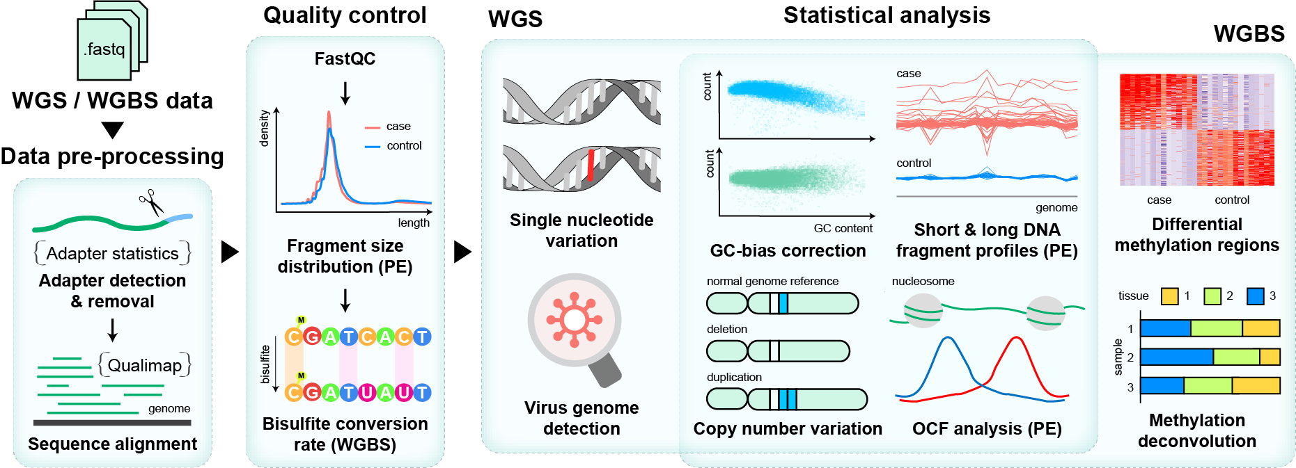
The whole pipeline is established based on the processing graph principle. Users can use the preset pipeline for WGBS/WGS data as well as build their own analysis pipeline from any intermediate data like bam files. The main functions are as the following picture.
Section 1: Installation Tutorial
Section 1.1: System requirement
The popular WGBS/WGS analysis toolkits are released on Unix/Linux system, based on different program languages, like FASTQC and Bowtie2. Therefore, it’s very difficult to rewrite all the software in one language. Fortunately, conda/bioconda program collected many prevalent python modules and bioinformatics software, so we can install all the dependencies through conda/bioconda and arrange pipelines using python.
We recommend using conda/Anaconda and create a virtual environment to manage all the dependencies. If you did not install conda before, please follow this tutorial to install conda first.
After installation, you can create a new virtual environment for cfDNA analysis. Virtual environment management means that you can install all the dependencies in this virtual environment and delete them easily by removing this virtual environment.
Section 1.2: Create environment and Install Dependencies
We tested our pipeline using different versions of software and provide an environment yml file for users. Users can download this file and create the environment in one command line.
First, please download the yml file.
wget https://xwanglabthu.github.io/cfDNApipe/environment.yml
Then, run the following command. The environment will be created and all the dependencies as well as the latest cfDNApipe will be installed.
# clean unused packages before installation
conda clean -y --all

# install environment
conda env create -n cfDNApipe -f environment.yml
Note: The environment name can be changed by replacing “-n cfDNApipe” to “-n environment_name”.
Note: If errors about unavailable or invalid channel occur, please check that whether the .condarc file in your ~ directory had been modified. Modifing .condarc file may cause wrong channel error. In this case, just rename/backup your .condarc file. Once the installation finished, this file can be recoveried. Of course, you can delete .condarc file if necessary.
Section 1.3: Activate Environment and Use cfDNApipe
Once the environment is created, the users can enter the environment using the following command.
conda activate cfDNApipe
Now, just open python and process ** cell-free DNA WGBS/WGS paired/single end** data. For more detailed explanation for each function and parameters, please see cfDNApipe documentation.
Section 2: cfDNApipe Highlights
cfDNApipe is a highly integrated cfDNA WGS/WGBS data processing pipeline. We designed many useful build-in mechanisms. Here, we will introduce some important features.
Section 2.1: Dataflow Graph for WGS and WGBS Data Processing
cfDNApipe is organized by a built-in dataflow with a strictly defined up- and down-stream data interface. The following figure shows how WGS and WGBS data are processed.
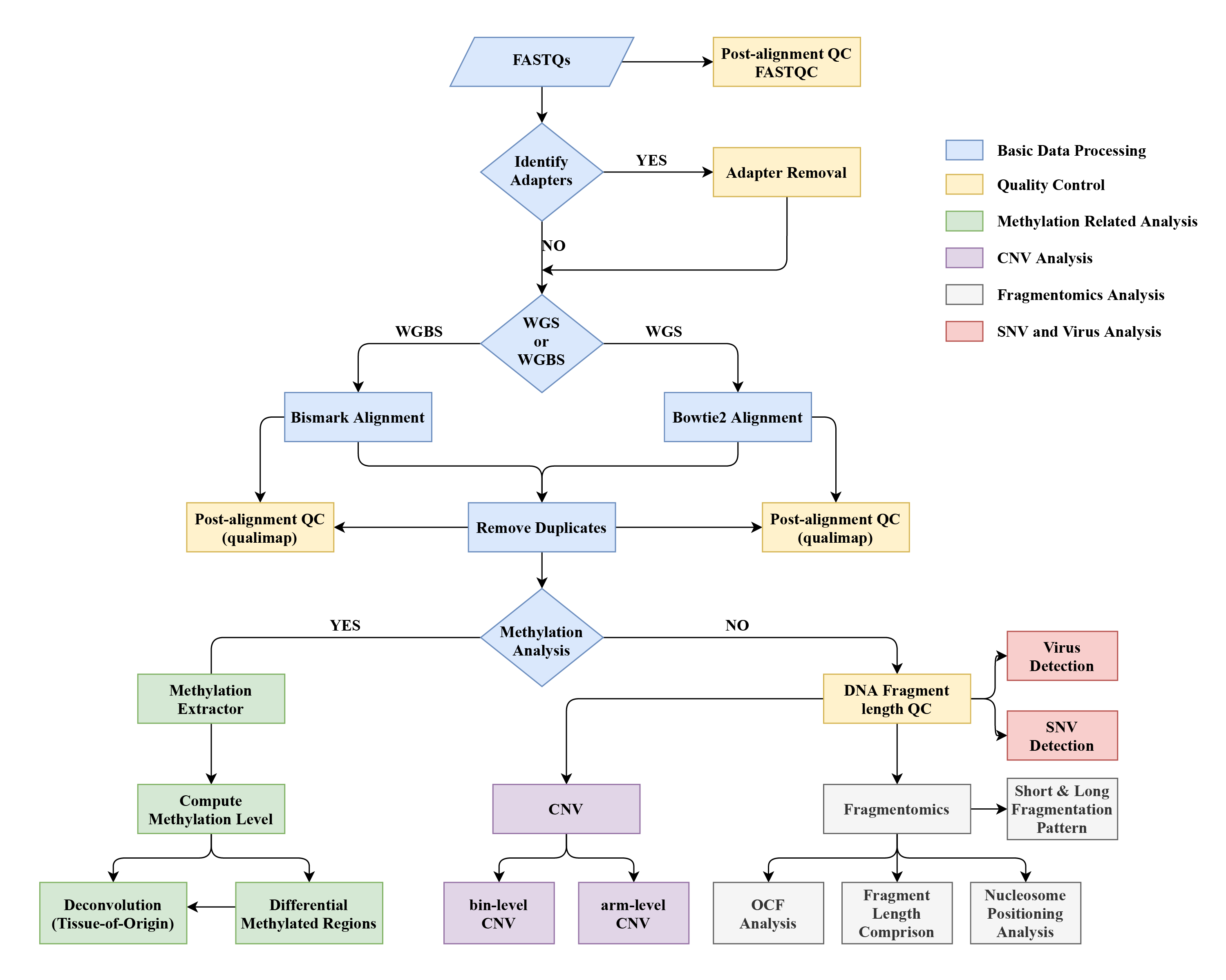
For detailed data flow diagrams, please see this cfDNApipe documentaion. In this documentation, we give thorough up- and down-stream relationships for every step.
Section 2.2: Reference Auto Download and Building
For any HTS data analysis, the initial step is to set reference files such as genome sequence and annotation files. cfDNApipe can download references and build reference indexes automatically. If the reference and index files already exist, cfDNApipe will use these files instead of download or rebuilding.
What reference files does cfDNApipe need?-
For analyzing WGS data (taken hg19 as example) genome sequence file and indexes: hg19.fa, hg19.chrom.sizes, hg19.dict, hg19.fa.fai bowtie2 related files: hg19.1.bt2 ~ hg19.4.bt2, hg19.rev.1.bt2~ hg19.rev.2.bt2 Other reference files: like blacklist file and cytoBand file, we provide them here.
-
For analyzing WGBS data (taken hg19 as an example) genome sequence file and indexes: hg19.fa, hg19.chrom.sizes, hg19.dict, hg19.fa.fai bismark related files: Bisulfite_Genome folder with CT_conversion and GA_conversion Other reference files: like CpG island file and cytoBand file, we provide them here.
Here, we introduced the global reference configure function in cfDNApipe to download and build reference files automatically.
cfDNApipe contains 2 types of global reference configure function, pipeConfigure and pipeConfigure2. Function pipeConfigure is for single group data analysis (without control group). Function pipeConfigure2 is for case and control analysis. Either function will check the reference files, such as bowtie2 and bismark references. If not detected, references will be downloaded and built. This step is necessary and puts things right once and for all.
Note: Users should use the correct configure function pipeConfigure and pipeConfigure2. The output folder arrangement strategy is different for these two functions. In addition, some default files can only be accessed through pipeConfigure or pipeConfigure2. Therefore, if a single group data analysis is needed, use pipeConfigure and Configure. If a case-control comparison analysis is needed, using pipeConfigure2 and Configure2. If users want to switch analysis from a single group to a case-control group and vice versa, the customized pipeline can achieve the seamless linking between output and input of different functions.
The following is a simple pipeConfigure example for building WGBS reference files.
from cfDNApipe import *

pipeConfigure(
    threads=60,
    genome="hg19",
    refdir=r"path_to_reference/hg19_bismark",
    outdir=r"path_to_output/WGBS",
    data="WGBS",
    type="paired",
    JavaMem="10g",
    build=True,
)
pipeConfigure function takes 8 necessary parameters as input.
- ‘threads’: the max threads user want to be used.
- ‘genome’: which genome to be used, must be ‘hg19’ or ‘hg38’.
- ‘refdir’: where to find genome reference files like sequence fasta file and CpG island ananotation files.
- ‘outdir’: where to put all the output files.
- ‘data’: “WGBS” or “WGS”.
- ‘type’: “paired” or “single”.
- ‘JavaMem’: maximum memory java program can used.
- ‘build’: download and build reference or not after reference checking.
Like the above example, if refdir is empty, cfDNApipe will download hg19.fa and other annotation files automatically. Once done, the program will print “Background reference check finished!”, then users can do the analyzing steps.
-
How to use local reference files?
The download procedure is always time-consuming. cfDNApipe can detect the reference files which are already existed in refdir. Therefore, users can employ already established references without rebuilding. For instance, users can just put hg19.fa and bowtie2 related files into refdir and cfDNApipe will not download and rebuild them again. Other reference files can be got from here. Downloading, uncompressing and putting them into refdir will be much faster.
We also provide a simple pipeConfigure2 example for building WGBS reference files.
from cfDNApipe import *

pipeConfigure2(
    threads=60,
    genome="hg19",
    refdir=r"path_to_reference/hg19_bismark",
    outdir=r"path_to_output/WGBS",
    data="WGBS",
    type="paired",
    case="cancer",
    ctrl="normal",
    JavaMem="10g",
    build=True,
)
- ‘case’: Case group name flag.
- ‘ctrl’: Control group name flag.
Section 2.3: Output Folder Arrangement
Generally, cell-free DNA analysis contains many steps, which will generate lots of output files. cfDNApipe arranges the outputs into every functional-specific folder. Based on the analysis strategy (with or without control), the output folders are arranged as follows.
- Analysis Results Without Control Samples
output_folders/
├── final_result/
├── report_result/
│   ├── Cell_Free_DNA_WGBS_Analysis_Report.html
│   └── Other files and folders
└── intermediate_result/
    ├── step_01_inputprocess
    ├── step_02_fastqc
    ├── step_02_identifyAdapter
    └── Other processing folders
- Analysis Results With Control Samples (assume case and control)
output_folders/
├──case/
│   ├── final_result/
│   ├── report_result/
│   │   ├── Analysis_Report.html
│   │   └── Other files and folders
│   └── intermediate_result/
│       ├── step_01_inputprocess
│       ├── step_02_fastqc
│       ├── step_02_identifyAdapter
│       └── Other processing folders
├──control/
    ├── final_result/
    ├── report_result/
    │   ├── Analysis_Report.html
    │   └── Other files and folders
    └── intermediate_result/
        ├── step_01_inputprocess
        ├── step_02_fastqc
        ├── step_02_identifyAdapter
        └── Other processing folders
There will be 3 major ouput folder for every sample group, named “intermediate_result”, “report_result”, and “final_result”.
Folder “intermediate_result” contains folders named by every single step, all the intermediate results and processing records will be saved in each folder. Users can access any files they want. This folder is very large since all the intermediate files are saved in this folder. Users can move some results to the folder “final_result” and deleted “intermediate_result” after all the analysis is finished.
Folder “report_result” save a pretty HTML report and related data which shows some visualization results like quality control and analysis figures. The report folder can be copied anywhere. Here is an example showing the final report.
Folder “final_result” is an empty folder for users to save specific results from the intermediate_result folder.
Section 2.4: Breakpoint Detection
Sometimes, the program may be interrupted by irresistible reasons like computer crashes. cfDNApipe provides breakpoint detection mechanism, which computes md5 code for inputs, outputs, as well as all parameters. Therefore, users do not worry about any interrupt situation. Re-running the same program, the finished step will show a message like below and be skipped automatically.
************************************************************
                bowtie2 has been completed!
************************************************************
Section 2.5: Other Mechanisms
- Parallel Computing
- Case and Control Analysis
- Inputs Legality Checking
- ……
Section 3: A Quick Tutorial for Analysis WGBS data
In this section, we will demonstrate how to perform a quick analysis for paired-end WGBS data using the build-in pipeline.
Section 3.1: Set Global Reference Configures
First, users must set some important configure, for example, which genome to be used, how many threads should be used and where to put the analysis results. cfDNApipe provides a configure function for the users to set these parameters. Below is an instance.
from cfDNApipe import *

pipeConfigure(
    threads=60,
    genome="hg19",
    refdir=r"path_to_reference/hg19_bismark",
    outdir=r"path_to_output/WGBS",
    data="WGBS",
    type="paired",
    build=True,
    JavaMem="10g",
)
Section 3.2: Execute build-in WGBS Analysis Pipeline
cfDNApipe provides a preset pipeline for paired/single end WGBS/WGS data, user can use it easily by assigning fastq sequencing files as the input of the pipeline. All the parameters used in the pipeline are carefully selected after numerous tests.
res = cfDNAWGBS(inputFolder=r"path_to_fastqs",
                idAdapter=True,
                rmAdapter=True,
                dudup=True,
                CNV=False,
                armCNV=False,
                fragProfile=False,
                report=True,
                verbose=False)

# see all outputs
print(res)

# get a specific step
res.bismark

# output like below
<cfDNApipe.Fun_bismark.bismark object at 0x7effb860f438>

# get all output of a step
res.bismark.getOutputs()

# output like below
['outputdir', 'unmapped-1', 'unmapped-2', 'bamOutput', 'bismkRepOutput']

# get a spefic output
res.bismark.getOutput('bamOutput')

# output like below
[
'/opt/tsinghua/zhangwei/Pipeline_test/o_WGBS-PE/intermediate_result/step_04_bismark/case1.pair1.truncated.gz_bismark_bt2_pe.bam',
'/opt/tsinghua/zhangwei/Pipeline_test/o_WGBS-PE/intermediate_result/step_04_bismark/case2.pair1.truncated.gz_bismark_bt2_pe.bam',
'/opt/tsinghua/zhangwei/Pipeline_test/o_WGBS-PE/intermediate_result/step_04_bismark/case3.pair1.truncated.gz_bismark_bt2_pe.bam',
'/opt/tsinghua/zhangwei/Pipeline_test/o_WGBS-PE/intermediate_result/step_04_bismark/case4.pair1.truncated.gz_bismark_bt2_pe.bam'
]
#
*Note: If the error about “Java Can’t connect to X11 window server” occured, please remove the DISPLAY variable by the following command.
unset DISPLAY
In the above example, users just pass the input folder which contains all the raw fastq files (without any other files) to the function, then the processing will start and all results will be saved in the output folder mentioned in the former section. What’s more, “report=True” will generate an HTML report for users.
In addition, cfDNApipe also provides case-control comparison analysis for WGBS/WGS data. For using this function, please see the section 4 and function cfDNAWGS2 and cfDNAWGBS2.
Also, users can write the whole pipeline in a python file and run it in the backend like below.
nohup python WGBS_pipeline.py > ./WGBS_pipeline.log 2>&1 &
Section 4: Perform Case-Control Analysis for WGBS data
The analysis steps for case-control analysis are the same as section 3.1 and 3.2. First, set global configure. Second, run the analysis command.
Setting global configure is a little bit different from section 3.1. Below is an example.
from cfDNApipe import *

pipeConfigure2(
    threads=60,
    genome="hg19",
    refdir=r"path_to_reference/hg19_bismark",
    outdir=r"path_to_output/WGBS",
    data="WGBS",
    type="paired",
    JavaMem="10G",
    case="cancer",
    ctrl="normal",
    build=True,
)
Here, two more parameters are used. Parameter “case” and “ctrl” is the name flag for case and control data. These two parameters control the output for case and control samples.
Next, using function cfDNAWGBS2 to processing case and control analysis.
case_res, ctrl_res = cfDNAWGBS2(
    caseFolder=r"case_fastqs",
    ctrlFolder=r"ctrl_fastqs",
    caseName="cancer",
    ctrlName="normal",
    idAdapter=True,
    rmAdapter=True,
    dudup=True,
    armCNV=True,
    CNV=True,
    fragProfile=True,
    verbose=False,
)
After analysis, users can get all the output as well as reports for case and control. Of course, the comparison results will be saved in case folder.
If you want build customized pipeline in a case-control study, please use switchConfigure before any operation. switchConfigure function tells the program that the following steps should be saved in case or control specific folders. Below is a small demonstration. For a more detailed example, please see Section 6.3.
from cfDNApipe import *

# set all configures
pipeConfigure2(
    threads=60,
    genome="hg19",
    refdir=r"path_to_reference/hg19_bismark",
    outdir=r"path_to_output/WGBS",
    data="WGBS",
    type="paired",
    JavaMem="10G",
    case="cancer",
    ctrl="normal",
    build=True,
)

# switch to normal folder. If pipeConfigure2 is set but not calling any switchConfigure, there will report an error.
switchConfigure("normal")

# Here, do the analysis for normal samples

# switch to cancer folder. Without switchConfigure("cancer"), the analysis of cancer samples will saved in normal folder.
switchConfigure("cancer")

# Here, do the analysis for cancer samples

# switchConfigure can be used many time.
switchConfigure("normal")


switchConfigure("cancer")
Section 5: How to Build Customized Pipeline using cfDNApipe
Some users are familiar with cfDNA processing and want to customize their pipelines. cfDNApipe provides a flexible pipeline framework for building the customized pipeline. The following is an example of how to build the pipeline from intermediate steps.
Assume that we have some WGS samples and all the samples have already been aligned. Now, we want to perform CNA analysis to these data compared with the default sequence and get gene-level annotation.
First, set global configure.
from cfDNApipe import *
import glob

pipeConfigure(
    threads=60,
    genome="hg19",
    refdir=r"path_to_reference/hg19_bowtie2",
    outdir=r"path_to_output/WGS",
    data="WGS",
    type="paired",
    JavaMem="10G",
    build=True,
)
Second, take all the aligned bam as inputs.
# get all bam files
bams = glob.glob("samples/*.bam")

# sort bam and remove duplicates
res_bamsort = bamsort(bamInput=bams, upstream=True)
res_rmduplicate = rmduplicate(upstream=res_bamsort)

# perform CNV analysis, stepNum is set as flag of every step
res_cnvbatch = cnvbatch(
    caseupstream=res_rmduplicate,
    access=Configure.getConfig("access-mappable"),
    annotate=Configure.getConfig("refFlat"),
    stepNum="CNV01",
)
res_cnvPlot = cnvPlot(upstream=res_cnvbatch, stepNum="CNV02")
res_cnvTable = cnvTable(upstream=res_cnvbatch, stepNum="CNV03")
res_cnvHeatmap = cnvHeatmap(upstream=res_cnvbatch, stepNum="CNV04")
In the above codes, “upstream=True” means puts all the results to the well-arranged output folder.
Also, sophisticated users can change computational resources in every step using Configure (for single group samples) and Configure2 (for case-control samples) like below.
# see all methods in Configure
dir(Configure)

# output like below
['_Configure__config', '__class__', '__delattr__', '__dict__',
'__dir__', '__doc__', '__eq__', '__format__', '__ge__', '__getattribute__',
'__gt__', '__hash__', '__init__', '__init_subclass__', '__le__', '__lt__',
'__module__', '__ne__', '__new__', '__reduce__', '__reduce_ex__',
'__repr__', '__setattr__', '__sizeof__', '__str__', '__subclasshook__',
'__weakref__', 'bismkrefcheck', 'bt2refcheck', 'checkFolderPath',
'configureCheck', 'genomeRefCheck', 'getConfig', 'getConfigs', 'getData',
'getFinalDir', 'getGenome', 'getJavaMem', 'getOutDir', 'getRefDir',
'getRepDir', 'getThreads', 'getTmpDir', 'getTmpPath', 'getType',
'gitOverAllCheck', 'githubIOFile', 'pipeFolderInit', 'refCheck',
'setConfig', 'setData', 'setGenome', 'setJavaMem', 'setOutDir',
'setRefDir', 'setThreads', 'setType', 'snvRefCheck', 'virusGenomeCheck']

# get all parameters
Configure.getConfigs()

# output like below
dict_keys(['threads', 'genome', 'refdir', 'outdir', 'tmpdir', 'finaldir',
'repdir', 'data', 'type', 'JavaMem', 'genome.seq', 'genome.idx.fai',
'genome.idx.dict', 'chromSizes', 'CpGisland', 'cytoBand', 'OCF',
'PlasmaMarker', 'Blacklist', 'Gaps', 'refFlat', 'access-mappable'])

# change threads
Configure.setThreads(20)

# change threads in another way
Configure.setConfig("threads", 20)
Section 6: A Basic Quality Control: Fragment Length Distribution
The fragment length distribution of cfDNA contains important information like nucleosome positioning and tissue-of-origin. For example, Jahr et al. found that DNA fragments produced by apoptosis illustrate peaks around 180bp and its multiples, whereas necrosis results in much longer fragments. Snyder, et al. report the fragment length peaks corresponding to nucleosomes (~147 bp) and chromosomes (nucleosome + linker histone; ~167 bp). Besides, based on Mouliere, et al. and Jiang, et al., necrosis results in much longer fragments, usually > 1000bp. Therefore, longer fragments may reveal the signal from necrosis.
In this section, we will show how to generate fragment length distribution figures and related statistics.
Note: Be aware that default parameters in alignment is set to filter reads longer than 500bp. Therefore, if users want to remain these reads, set "-X" in bowtie2 and bismark class. For example, other_params={"-X": 2000} means that the maximum insert size for valid paired-end alignments is 2000bp.
we taken only 4 example from Snyder, et al. as an example.
from cfDNApipe import *
import glob
import pysam

pipeConfigure(
    threads=20,
    genome="hg19",
    refdir=r"path_to_reference/hg19_bowtie2",
    outdir=r"path_to_output/WGS",
    data="WGS",
    type="paired",
    JavaMem="10G",
    build=True,
)

verbose = False

case_bed = ["./HCC/GM1100.bed", "./HCC/H195.bed"]
ctrl_bed = ["./Healthy/C309.bed", "./Healthy/C310.bed"]

res_fraglenplot_comp = fraglenplot_comp(
    casebedInput=case_bed, ctrlbedInput=ctrl_bed, ratio1=150, ratio2=400,
    caseupstream=True, verbose=verbose)
We can get the following figure and a txt file named “statistic.txt”
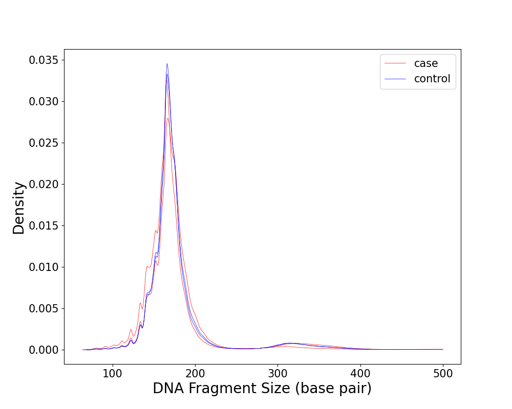
	                Short(<150 bp) Rate	Long(>400 bp) Rate	Peak 1	Peak 2
GM1100_fraglen.pickle	0.19611894376561956	0.0018909480762622482	165	330
H195_fraglen.pickle	0.1177497441211625	0.0048737613946009	167	334
C309_fraglen.pickle	0.11525248298337597	0.0034377031387753682	166	332
C310_fraglen.pickle	0.11717840394001733	0.0033180126814695457	166	332
The result shows that all the sample has a peak around ~167bp and HCC patients have more short fragments than the healthy, which are consistent with Mouliere, et al..
If users want to analysis cfDNA from necrosis, please use parameters "other_params={"-X": 2000}" in bismark or bowtie2 and "ratio2=1000" for ploting fragment length distribution. This will report proportion of cfDNA longer than 1000bp which may come from necrosis.
Section 7: Nucleosome Positioning
Note: This function is only supported for processing WGS data.
Snyder, et al. reports that the intensity of the FFT signal of nucleosome positioning around gene body is correlated with gene expression at specific frequency ranges, with a maximum at 177–180 bp for positive correlation and a minimum at ~199 bp for the negative correlation. Therefore, nucleosome positioning is an important feature for identifying cfDNA origin. Researchers proposed a statistics named windowed protection score (WPS) to reveal the nucleosome positioning in cfDNA HTS data. cfDNApipe provides the function to calculate WPS in any genome region. The following steps illustrate how to compute WPS in arbitrary genome regions.
First, select the genome regions.
Snyder, et al. selected the first 10 kb of gene bodies. However, TF binding regions also show different signals compared with the flanking region. TF binding regions are changed in different cell types and different cell states and gene annotation is updating continuously. Therefore, cfDNApipe does not provide a pre-set region file instead of telling the users how to get the genome regions from gencode annotation files.
In this part, we will illustrate how to get gene bodies from gencode annotation files.
Users can download gencode annotation files from gencode database, the commonly used files are gencode.v19.annotation.gtf.gz for hg19 and gencode.v37.annotation.gtf.gz for hg38. Here, we use hg19 as an example.
library(rtracklayer)
library(dplyr)

anno_raw <- import("gencode.v19.annotation.gtf.gz")

# get all genes
anno_raw <- anno_raw[which(anno_raw$type == "gene"), ]

anno <- data.frame(gene_id = anno_raw$gene_id, chr = seqnames(anno_raw),
                   start = start(anno_raw), end = end(anno_raw),
                   strand = strand(anno_raw))

# get genome region downstream 10000bp from TSS
for (i in nrow(anno)) {
    if (anno$strand[i] == "+") {
        anno$start = anno$start - 1
        anno$end = anno$start + 10000
    } else {
        anno$start =anno$end + 1 - 10000
        anno$end = anno$end + 1
    }
}

# remove invalid
anno <- anno[which(anno$chr %in% paste0("chr", c(1:22, "X"))), ]
anno <- anno[which(anno$start > 0), ]

write.table(x = anno, file = "transcriptAnno-v19.tsv", sep = "\t",
            col.names = FALSE, row.names = FALSE, quote = FALSE)
Note: Be aware of the feature number in your annotation file. From the above Rscript, 57820 genes remained. Users should filter the features such as protein-coding genes. Linux system limits file number in a folder, therefore, shrink the rows in the annotation file is necessary.
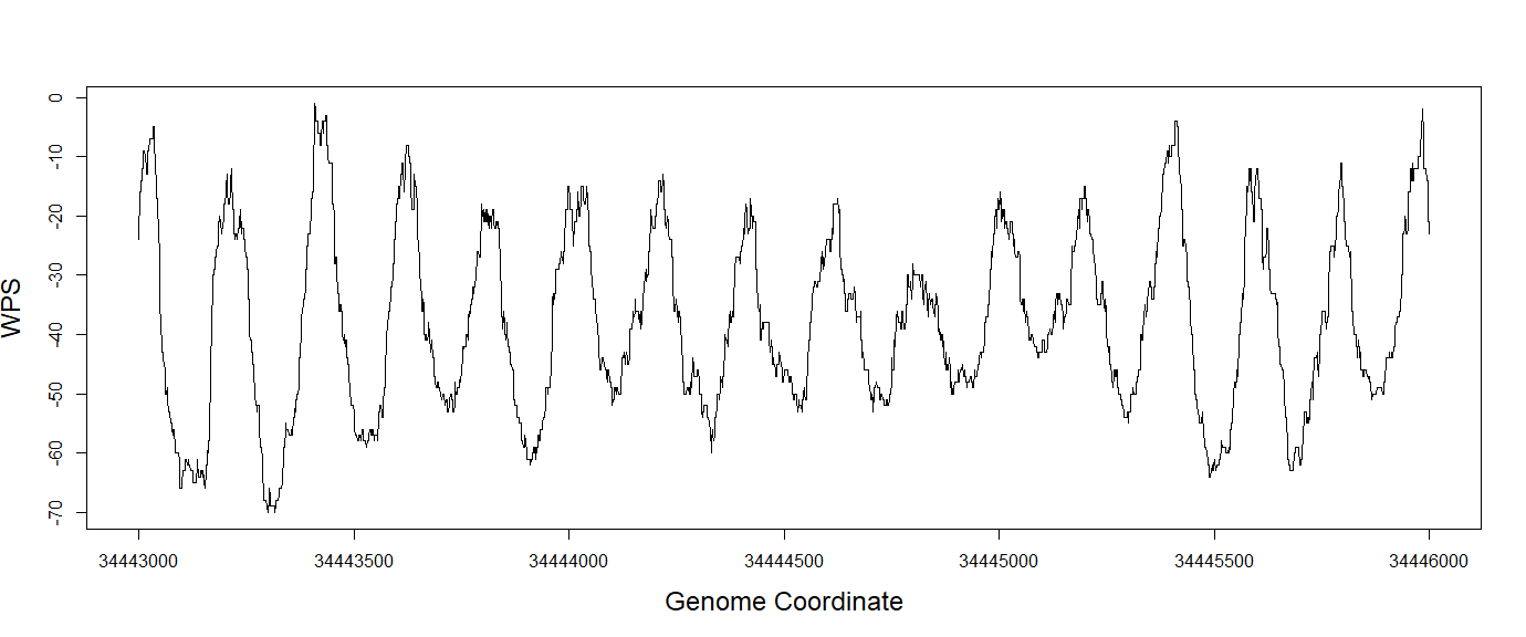
From the above code, users can get a tsv file named “transcriptAnno-v19.tsv” which saves the genome region downstream 10000bp from gene TSS. Users can get customized regions like TF binding regions. For a better illustration, we added one region at the end of “transcriptAnno-v19.tsv”. This region is from the alpha-satellite region in chr12 which shows a strongly positioned nucleosomes signal reported by Snyder, et al..
alpha_satellite chr12 34443000 34446000 +
Second, compute WPS for these regions. Low coverage sample shows weak WPS signal, therefore, we use one sample IC17 (Hepatocellular Carcinoma, 42.08X coverage) from Snyder, et al. for better illustration. Users can perform the following analysis by using the pre-set pipeline results or aligned bam files from the customized script.
from cfDNApipe import *

pipeConfigure(
    threads=60,
    genome="hg19",
    refdir="/home/zhangwei/Genome/hg19_bowtie2",
    outdir="/opt/tsinghua/zhangwei/nucleosome_positioning",
    data="WGS",
    type="paired",
    JavaMem="8G",
    build=True,
)

# be aware all the samples should in a list
res1 = bam2bed(bamInput=["SRR2130016-rmdup.bam"], upstream=True)

res2 = runWPS(upstream=res1, tsvInput="transcriptAnno-v19.tsv")
We can find the output files saved in the folder “intermediate_result/step_02_runWPS/SRR2130016.bed” and plot the WPS like below.
data <- read.table("SRR2130016.bed_alpha_satellite.tsv.gz")
WPS <- data$V5

x <- seq(34443000, 34446000)

plot(x = x, y = WPS, type = "l",
     xlab = "genome coordinate", ylab = "WPS", lwd = "1")
For the following analysis like FFT and correlation with gene expression, this analysis is highly user-specific and can be easily performed from the results of cfDNApipe.
Section 8: Inferring Tissue-Of-Origin based on deconvolution
Inferring tissue-of-origin from cfDNA data is of great potential for further clinical applications. For example, as Fiala, et al. mentioned, cancerous cells release more DNA into plasma. Therefore, inferring tissue-of-origin can be used for early cancer detection. In cfDNApipe, tissue-of-origin analysis can be achieved through OCF analysis or deconvolution.
Sun, et al. proposed a deconvolution strategy for inferring tissue proportion from WGBS data. Moss, et al. also exhibits the feasibility of this. We collected WGBS data of plasma cfDNA from 32 healthy people and 24 HCC patients (A and B stage) applied a novel deconvolution algorithm on this dataset to infer the fraction of liver-derived cfDNA in each sample by using an external methylation reference from Sun, et al..
The basic analysis can be achieved by using the pre-set pipeline. Here, we start with the extracted methylation files.
First, set global parameters and compute methylation level for regions from Sun, et al.. The deconvolution can be accomplished using only one command in python.
import glob
from cfDNApipe import *

pipeConfigure2(
    threads=100,
    genome="hg19",
    refdir=r"path_to_reference/hg19_bismark",
    outdir=r"path_to_output/WGBS",
    data="WGBS",
    type="single",
    case="HCC",
    ctrl="Healthy",
    JavaMem="10G",
    build=True,
)

hcc = glob.glob("/WGBS/HCC/intermediate_result/step_06_compress_methyl/*.gz")
ctr = glob.glob("/WGBS/Healthy/intermediate_result/step_06_compress_methyl/*.gz")

verbose = False

switchConfigure("HCC")
hcc1 = calculate_methyl(tbxInput=hcc, bedInput="plasmaMarkers_hg19.bed", upstream=True, verbose=verbose)
hcc2 = deconvolution(upstream=hcc1)

switchConfigure("Healthy")
ctr1 = calculate_methyl(tbxInput=ctr, bedInput="plasmaMarkers_hg19.bed", upstream=True, verbose=verbose)
ctr2 = deconvolution(upstream=ctr1)
Note: The default bedInput for class calculate_methyl is CpG island regions. Therefore, we should change this file to match the external reference provided in cfDNApipe. Of course, user-defined files can be passed to deconvolution easily. For detailed parameter explanation, please see here.
Next, plot liver proportion between HCC patients and healthy people in R.
library(ggplot2)

HCC <- read.table(file = "path_to_output/WGBS/Healthy/intermediate_result/step_02_deconvolution/result.txt", header = TRUE, sep = "\t", row.names = 1)
CTR <- read.table(file = "path_to_output/WGBS/HCC/intermediate_result/step_02_deconvolution/result.txt", header = TRUE, sep = "\t", row.names = 1)

HCC.liver <- unlist(HCC["Liver", ])
CTR.liver <- unlist(CTR["Liver", ])
p <- wilcox.test(x = CTR.liver, y = HCC.liver, alternative = "less")$p.value

data <- data.frame(Class = c(rep("Healthy", 32), rep("HCC", 24)),
                     Liver_Prop = c(CTR.liver, HCC.liver))

ggplot(data, aes(x=Class, y=Liver_Prop, fill=Class)) +
    geom_boxplot() +
    labs(x = paste("T-TEST:", p, sep = " ")) +
    labs(y = "Liver Proportion") +
    theme(axis.text.x = element_text(size = 16)) +
    theme(axis.title = element_text(size = 16)) +
    theme(legend.text = element_text(size = 16)) +
    theme(title = element_text(size = 16)) +
    theme(axis.text = element_text(size = 16)) +
    theme(panel.grid.major = element_blank(),
          panel.grid.minor = element_blank(),
          panel.background = element_blank(),
          axis.line = element_line(colour = "black"),
          panel.border = element_rect(colour = "black", fill=NA, size=2))
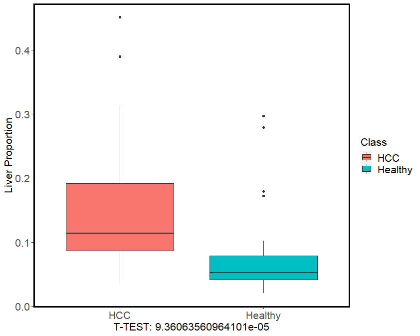
The result is like the following figure. cfDNApie estimated higher liver-derived fractions in cfDNA from HCC patients with an average value of 15.2%, while those from healthy people with an average value of 7.6%. The liver-derived fractions in cfDNA between HCC patients and healthy people show a significant statistical difference (Mann–Whitney U test, p-value =9.36×10⁻⁵), which is consistent with the Sun, et al.. The results suggest that cfDNApipe has the potential to infer tissue-of-origin and detect changes of proportions from different tissues.
Section 9: Additional Function: WGS SNV/InDel Analysis
Note: This function is only supported for processing WGS data.
Section 9.1: Sequencing Coverage for Analyzing Mutation in cfDNA WGS Data
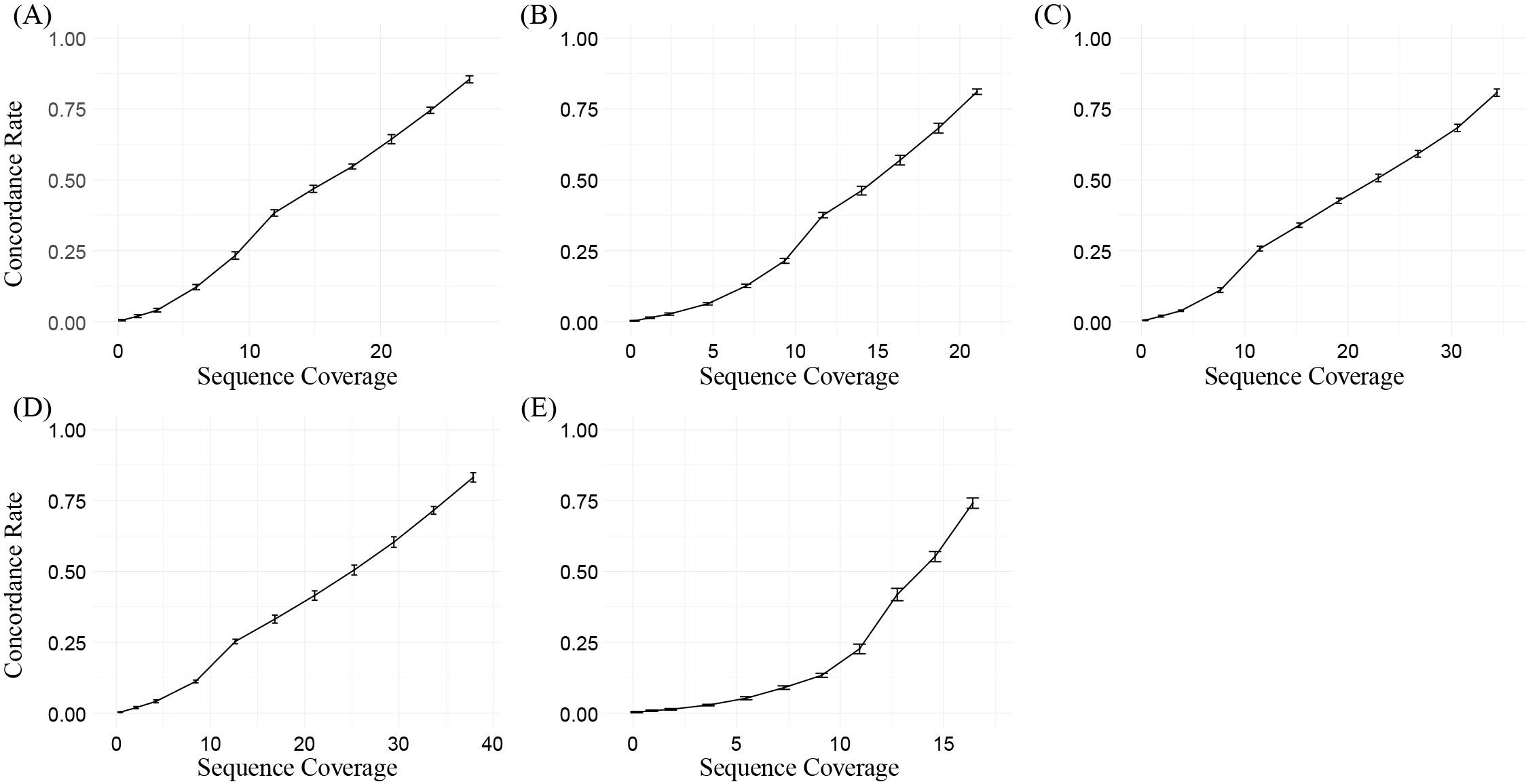
The performance of SNV detection is largely influenced by the sequencing coverage in cfDNA WGS data. In general, lower sequencing coverage will lead to a higher undetected rate. Chen, et al. compared Strelka2 and Mutect2 (GATK tool, cfDNApipe adopted method) and found that Mutect2 performed better when the mutation frequency was lower than 10%. Mauger, et al. has proved that both germline and somatic mutations can be detected using the GATK tool at 10X or 30X sequencing coverage in cfDNA. We selected 5 deep sequenced samples (IC15, Lung cancer, 29.77X; IC17, Liver cancer, 42.08X; IC20, Lung cancer, 23.38X; IC35, Breast cancer, 18.22X; IC37, Colorectal cancer, 38.22X) from Snyder, et al., and performed a down-sampling simulation in chr20. As Kishikawa, et al. did, we evaluated the concordance of somatic mutations and gene-level CNVs between the down-sampled data and the WGS data using all the sequence reads. Here, we take IC17 as an example and all the simulation code can be found here.
First, down-sampling IC17 using samtools.
# Downsample command
# variable i is random seed, variable ratio is used to control sequencing coverage
samtools view -bhs $i"."$ratio -o "IC17_"$ratio"_"$i".bam" IC17_chr10.bam
Then, run cfDNApipe to detect somatic mutaion.
from cfDNApipe import *
import argparse
import os

pipeConfigure(
    threads=10,
    genome="hg19",
    refdir="path_to_ref/hg19_bowtie2",
    outdir="path_to_each_output",
    data="WGS",
    type="paired",
    JavaMem="10G",
    build=True,
)

# check SNV reference path
Configure.snvRefCheck(folder="/home/zhangwei/Genome/SNV_hg19", build=True)

bams = [args.input]

# Using bam files directly.
# Of course, the "upstream" of addRG can be from "rmduplicate".
res1 = addRG(bamInput=bams, upstream=True)

res2 = BaseRecalibrator(upstream=res1, knownSitesDir=Configure.getConfig("snv.folder"))
res3 = BQSR(upstream=res2)
res4 = getPileup(upstream=res3, biallelicvcfInput=Configure.getConfig("snv.ref")["7"],)
res5 = contamination(upstream=res4)

res6 = mutect2t(
    caseupstream=res5, vcfInput=Configure.getConfig("snv.ref")["6"], ponbedInput=Configure.getConfig("snv.ref")["8"],
)

# res7 = filterMutectCalls(upstream=res6, other_params = {"--f-score-beta": 0.5})
res7 = filterMutectCalls(upstream=res6)
res8 = gatherVCF(upstream=res7)

# split somatic mutations
res9 = bcftoolsVCF(upstream=res8, stepNum="somatic")
Finally, We selected somatic SNV and compute precision and recall using R. The detected somatic mutation file is taken as input.
Note: Here, we chose a stric threshold “TLOD>4” for selecting the positive mutation. Users also can use frequency as thresholds to select valid muations. For detailed information about how to set threshold, please see here.
library(vcfR)
library(tidyr)
library(GenomicRanges)
library(gridExtra)
library(ggplot2)
library(stringr)

TLOD_filter <- function (vcf.file, threshold, makeGR = FALSE) {
    vcf.data <- read.vcfR(vcf.file)
    vcf.data <- as.data.frame(vcf.data@fix)
    vcf.data <- separate(data = vcf.data, col = INFO, into = c("INFO", "TLOD"), sep = ";TLOD=")
    vcf.data <- vcf.data[which(as.numeric(vcf.data$TLOD) > threshold), ]
    if (nrow(vcf.data) == 0) {
        return(GRanges())
    } else {
        if (makeGR == TRUE) {
            vcf.data <- vcf.data[c("CHROM", "POS", "POS")]
            colnames(vcf.data) <- c("chr", "start", "end")
            vcf.data <- makeGRangesFromDataFrame(vcf.data)
        }

        return(vcf.data)
    }

}

samples <- c("IC15", "IC17", "IC20", "IC35", "IC37")
covs <- c(29.77, 42.08, 23.38, 18.22, 38.22)

# Threshold is set to 4
threshold <- 4

df.summary <- list()

for (ll in seq(5)) {
    sample <- samples[ll]
    cov <- covs[ll]

    path <- paste0("./", sample, "/SNV/")

    # create granges
    chr20 <- TLOD_filter(vcf.file = paste0(path, "chr20/intermediate_result/step_somatic_bcftoolsVCF/", sample, "_chr20.somatic.vcf.gz"),
                         threshold = threshold, makeGR = TRUE)

    count.concordance <- list()

    for (i in c("01", "05", seq(9))) {
        this.concordance <- c()
        for (j in seq(10)) {
            vcf.file <- paste0(path, "ds_", i, "_", j, "/intermediate_result/step_somatic_bcftoolsVCF/", sample, "_", i, "_", j, ".somatic.vcf.gz")
            print(vcf.file)
            this.vcf <- TLOD_filter(vcf.file = vcf.file, threshold = threshold, makeGR = TRUE)
            # TP + FP
            this.allcount <- length(this.vcf)
            # TP
            this.TP <- sum(countOverlaps(query = chr20, subject = this.vcf))
            # FN
            this.FN <- length(chr20) - this.TP
            # FP
            this.FP <- this.allcount - this.TP
            # concordance
            tmp_concordance <- this.TP / (this.TP + this.FP + this.FN)
            this.concordance <- c(this.concordance, tmp_concordance)
        }
        name <- paste0("ds_", i)
        count.concordance[[name]] <- this.concordance
    }

    m.concordance <- unlist(lapply(count.concordance, mean))
    s.concordance <- unlist(lapply(count.concordance, sd))

    # only concordance rate
    df.sample <- data.frame(m.concordance = m.concordance, s.concordance = s.concordance,
                            cov = c(0.01, 0.05, seq(0.1, 0.9, 0.1)) * cov)

    df.summary[[sample]] <- df.sample
}


saveRDS(object = df.summary, file = paste0("SNV_", threshold, ".RDS"))
Finally, plot concordance rate curve.
library(ggplot2)
library(gridExtra)
library(tidyverse)
library(wesanderson)
library(dplyr)

data <- readRDS("SNV_4.RDS")

plot_lst <- vector("list")

for (i in seq(length(data))) {
    name <- names(data)[i]
    df.sample <- data[[name]]

    p1 <- ggplot(df.sample, aes(x=cov, y=m.concordance)) +
        geom_line(size=1) +
        geom_point(size=1)+
        geom_errorbar(aes(ymin=m.concordance-s.concordance, ymax=m.concordance+s.concordance),
                      width=0.6, size=1,
                      position=position_dodge(0)) +
        theme_minimal() +
        xlim(-0.5, max(df.sample$cov) + 1) +
        ylim(0, 1) +
        xlab("Sequence Coverage") +
        ylab("Concordance") +
        theme(axis.text.x = element_text(size = 13),
              axis.text.y = element_text(size = 13),
              axis.title.x = element_text(size = 18),
              axis.title.y = element_text(size = 18),
              legend.text = element_text(size=12))

    plot_lst[[i]] <- p1
}

fi.fig <- marrangeGrob(plot_lst, nrow = 2, ncol = 3)

# fi.fig

ggsave(filename = "SNV_plot.pdf", plot = fi.fig, width = 750, height = 350, units = "mm")
In fact, there are still some other challenges such as PCR amplification and sequencing error which could lead to false-positive results in cfDNA WGS data. Thus, whole-genome sequencing may not be the most suitable way to detect disease-related somatic mutations. For reliable clinical usage, panel- or UMI-based strategies are more preferred. The aim that we integrated mutation detection functions into cfDNApipe is to provide information contained in cfDNA as much as possible to help users grasp the mutation landscape as well as discover possible somatic mutations.
In conclusion, combined with the simulation results and Mauger, et al., we recommend at least 15X sequencing depth (average concordance rate 0.441 across all simulation samples) for preliminary detection, and higher depths are welcome for more accurate detection.
CNV detection in low coverage data is also challenging. We performed the same simulation as mutation detection.The similar simulation about CNV can be found here.
Threshold parameters in CNV detection: The main threshold parameters are “–target-avg-size” in function “cnvbatch” and “–threshold”, “–min-probes” in function “cnvTable”.
-
”–target-avg-size”: Increase the “target” average bin size (–target-avg-size), e.g. to at least 1000 bases for 30x coverage, or proportionally more for lower-coverage sequencing.
-
”–threshold”: A threshold of .2 (the default) will report single-copy gains and losses in a completely pure tumor sample (or germline CNVs), but a lower threshold would be necessary to call somatic CNAs if significant normal-cell contamination is present.
-
”–min-probes”: Some likely false positives can be eliminated by dropping CNVs that cover a small number of bins, at the risk of missing some true positives. With -m 3, the default, genes where only 1 or 2 bins show copy number change will not be reported.
The following result is the same simulation for CNV detection.
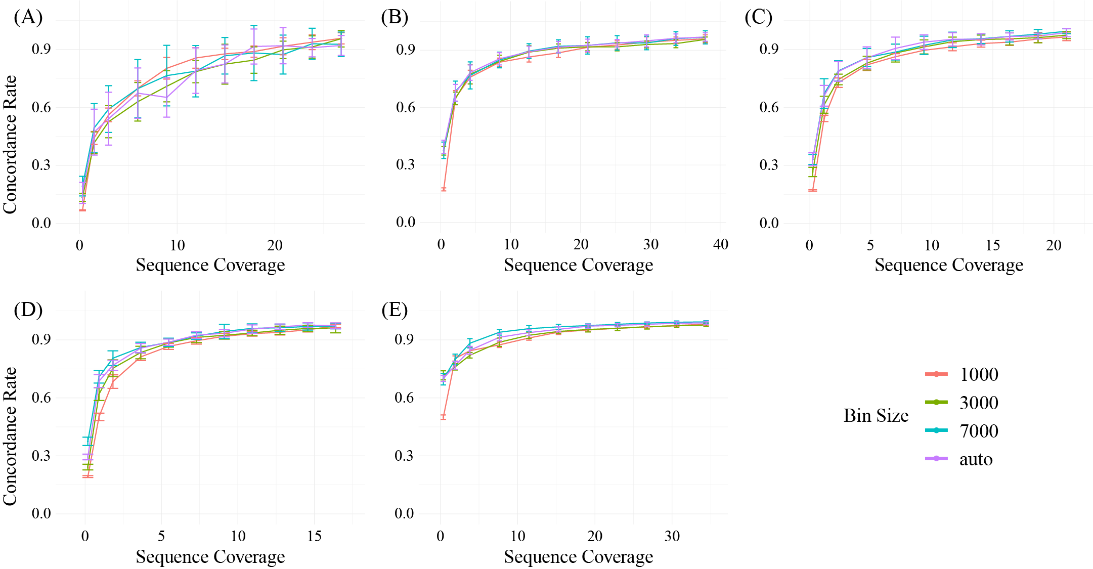
we recommend 5X coverage (average concordance rate 0.795 across all simulation samples) for the CNV detection using cfDNApipe. In addition, we strongly recommend users to try a larger bin size when the sequencing coverage is low for CNV detection as the tutorial of cnvkit recommended.
Section 9.2: Reference Files Preparation
We wrapped classical software GATK4 to call WGS mutations. Detecting mutations needs additional references related to the human genome. These references are provided by GATK resource bundle and not suit for auto-downloading. Therefore, users should download the reference files manually. GATK resource bundle provides different ways to download reference files like lftp and ftp. We recommend using lftp to download the VCF references for convenience.
If lftp is not installed, users can install it from conda easily.
conda install -c conda-forge lftp
Before the analysis, we recommend users creating a new folder for saving the snv related references files. For example, create a folder in your genome reference folder and name it based on the genome version like hg19_snv or hg38_snv. Then, enter the folder to download the snv reference files.
Users can login in GATK resource bundle and download the dependent VCF files.
lftp gsapubftp-anonymous@ftp.broadinstitute.org:/
#just click "Enter" for password
lftp gsapubftp-anonymous@ftp.broadinstitute.org:/> ls
Data hosted in GATK resource bundle is shown as follows.
drwxrwxr-x  12 ebanks   wga           235 Jul 30  2018 bundle
drwxrwxr-x   2 ebanks   wga           219 Nov 28  2011 DePristoNatGenet2011
drwxr-xr-x   2 droazen  broad         253 Oct 24  2014 foghorn140
-rw-r--r--   1 vdauwera broad     2141164 Jul 15  2014 gatkdocs-3_1_v_3_2.zip
drwxrwxr-x   2 ebanks   wga            34 Aug 12  2011 HLA
drwxrwxr-x   2 ebanks   wga           293 May 21  2019 Liftover_Chain_Files
-rw-r--r--   1 vdauwera broad    11645558 Aug  3  2017 mutect-1.1.7.jar
-rw-r--r--   1 vdauwera broad    10547264 Aug  3  2017 mutect-1.1.7.jar.zip
drwxrwxr-x   2 thibault broad         169 May 11  2015 travis
drwxrwxr-x   4 ebanks   wga            71 Aug  7  2016 triosForGA4GH
-rw-rw-r--   1 vdauwera broad    739681240 Oct 22  2013 tutorial_files.zip
drwxrwxr-x   7 vdauwera broad         126 Aug  3  2017 tutorials
drwxrwxr-x   5 vdauwera broad          72 Jun 24  2016 workshops
Then download the dependent files based on related genome version.
For hg19:
Note: Some files for hg19 is not provided by GATK, therefore we should convert them from b37 version. cfDNApipe will do the conversion automatically.
glob -- pget -c -n 12 bundle/hg19/1000G_omni2.5.hg19.sites.vcf.gz
glob -- pget -c -n 12 bundle/hg19/1000G_phase1.indels.hg19.sites.vcf.gz
glob -- pget -c -n 12 bundle/hg19/1000G_phase1.snps.high_confidence.hg19.sites.vcf.gz
glob -- pget -c -n 12 bundle/hg19/dbsnp_138.hg19.vcf.gz
glob -- pget -c -n 12 bundle/hg19/Mills_and_1000G_gold_standard.indels.hg19.sites.vcf.gz
glob -- pget -c -n 12 bundle/Mutect2/af-only-gnomad.raw.sites.b37.vcf.gz
glob -- pget -c -n 12 bundle/Mutect2/GetPileupSummaries/small_exac_common_3_b37.vcf.gz
glob -- pget -c -n 12 Liftover_Chain_Files/b37tohg19.chain
For hg38:
glob -- pget -c -n 12 bundle/hg38/1000G_omni2.5.hg38.vcf.gz
glob -- pget -c -n 12 bundle/hg38/1000G_phase1.snps.high_confidence.hg38.vcf.gz
glob -- pget -c -n 12 bundle/hg38/dbsnp_146.hg38.vcf.gz
glob -- pget -c -n 12 bundle/hg38/hapmap_3.3.hg38.vcf.gz
glob -- pget -c -n 12 bundle/hg38/Mills_and_1000G_gold_standard.indels.hg38.vcf.gz
glob -- pget -c -n 12 bundle/Mutect2/af-only-gnomad.hg38.vcf.gz.gz
glob -- pget -c -n 12 bundle/Mutect2/GetPileupSummaries/small_exac_common_3.hg38.vcf.gz
For analyzing single group samples, we need Public GATK Panel of Normals (PON) file. Here we provide the google storage download address directly.
For hg19, somatic-b37_Mutect2-WGS-panel-b37.vcf.
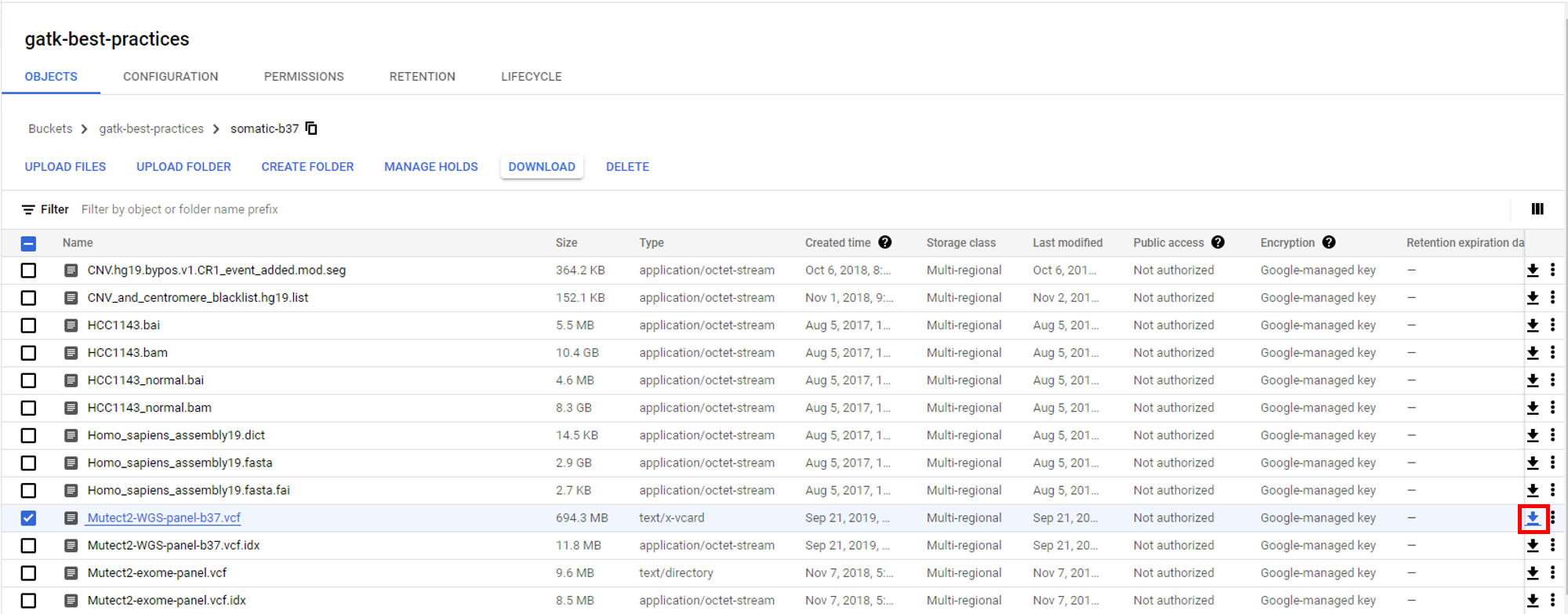
For hg38, somatic-hg38_1000g_pon.hg38.vcf.gz.
Just put the PON file in the same folder as the other snv reference files download before.
Finally, uncompressing all the files.
gunzip *.gz
Section 9.3: Performing Single Group Samples SNV Analysis
When finish preparing all the files, we can use “snvRefCheck” function in cfDNApipe to achieve genome version conversion from b37 to hg19 and indexing. Here we use hg19 to show the demo for single group samples SNV analysis.
The following are the whole scripts for single group samples SNV analysis with annotations.
from cfDNApipe import *
import glob

pipeConfigure(
    threads=60,
    genome="hg19",
    refdir=r"path_to_reference/hg19",
    outdir=r"path_to_output/snv_output",
    data="WGS",
    type="paired",
    build=True,
    JavaMem="10G",
)

# just set build=True to finish all the works
Configure.snvRefCheck(folder="path_to_reference/hg19/hg19_snv", build=True)

# see all the SNV related files
Configure.getConfig("snv.folder")
Configure.getConfig("snv.ref")

# indexed bam files after remove duplicates
bams = glob.glob("path_to_samples/*.bam")

res1 = addRG(bamInput=bams, upstream=True)

res2 = BaseRecalibrator(
    upstream=res1, knownSitesDir=Configure.getConfig("snv.folder")
)
res3 = BQSR(upstream=res2)

res4 = getPileup(
    upstream=res3,
    biallelicvcfInput=Configure.getConfig('snv.ref')["7"],
)

res5 = contamination(upstream=res4)

# In this step, files are split to chromatin
res6 = mutect2t(
    caseupstream = res5,
    vcfInput=Configure.getConfig('snv.ref')["6"],
    ponbedInput=Configure.getConfig('snv.ref')["8"],
)

#
res7 = filterMutectCalls(upstream=res6)

# put all chromatin files together
res8 = gatherVCF(upstream=res7)

# split somatic mutations
res9 = bcftoolsVCF(upstream=res8, stepNum="somatic")

# split germline mutations
res10 = bcftoolsVCF(
    upstream=res8, other_params={"-f": "'germline'"}, suffix="germline", stepNum="germline"
)
Note: User can adjust the parameter "--f-score-beta" in function filterMutectCalls for a very strict filtering. For detailed information, please see filterMutectCalls manual.
The output vcf file from function bcftoolsVCF can be annotated by other software such as annovar. Also, users can use IGV to visualize SNV in genome (link:Inspecting Variants in IGV).
Section 9.4: Performing Case-Control SNV Analysis
Here we also use hg19 to show the demo for case-control SNV analysis.
from cfDNApipe import *
import glob

# set global configure
pipeConfigure2(
    threads=100,
    genome="hg19",
    refdir=r"path_to_reference/hg19",
    outdir=r"path_to_output/snv_output",
    data="WGS",
    type="paired",
    case="cancer",
    ctrl="normal",
    JavaMem="10g",
    build=True,
)

Configure2.snvRefCheck(folder="path_to_reference/hg19/SNV_hg19", build=True)

case_bams = glob.glob("path_to_samples/cancer/*.bam")
ctrl_bams = glob.glob("path_to_samples/normal/*.bam")

# create PON file from normal samples
switchConfigure("normal")

ctrl_addRG = addRG(bamInput=ctrl_bams, upstream=True, stepNum="PON00",)
ctrl_BaseRecalibrator = BaseRecalibrator(
        upstream=ctrl_addRG,
        knownSitesDir=Configure2.getConfig("snv.folder"),
        stepNum="PON01",
        )
ctrl_BQSR = BQSR(upstream = ctrl_BaseRecalibrator, stepNum="PON02",)
ctrl_mutect2n = mutect2n(upstream = ctrl_BQSR, stepNum="PON03",)
ctrl_dbimport = dbimport(upstream = ctrl_mutect2n, stepNum="PON04",)
ctrl_createPon = createPON(upstream = ctrl_dbimport, stepNum="PON05",)

# performing comparison between cancer and normal
switchConfigure("cancer")
case_addRG = addRG(bamInput=case_bams, upstream=True, stepNum="SNV00",)
case_BaseRecalibrator = BaseRecalibrator(
    upstream=case_addRG,
    knownSitesDir=Configure2.getConfig("snv.folder"),
    stepNum="SNV01",
)

case_BQSR = BQSR(
    upstream=case_BaseRecalibrator,
    stepNum="SNV02")

case_getPileup = getPileup(
    upstream=case_BQSR,
    biallelicvcfInput=Configure2.getConfig('snv.ref')["7"],
    stepNum="SNV03",
)
case_contamination = contamination(
    upstream=case_getPileup,
    stepNum="SNV04"
)

# In this step, ponbedInput is ignored by using caseupstream parameter
case_mutect2t = mutect2t(
    caseupstream=case_contamination,
    ctrlupstream=ctrl_createPon,
    vcfInput=Configure2.getConfig('snv.ref')["6"],
    stepNum="SNV05",
)

case_filterMutectCalls = filterMutectCalls(
    upstream=case_mutect2t,
    stepNum="SNV06"
)

case_gatherVCF = gatherVCF(
    upstream=case_filterMutectCalls,
    stepNum="SNV07"
)

# split somatic mutations
case_somatic = bcftoolsVCF(upstream=case_gatherVCF, stepNum="somatic")

# split germline mutations
case_germline = bcftoolsVCF(
    upstream=case_gatherVCF, other_params={"-f": "'germline'"}, suffix="germline", stepNum="germline"
)
Note: User can adjust the parameter "--f-score-beta" in function filterMutectCalls for a very strict filtering. For detailed information, please see filterMutectCalls manual.
The output vcf file from function bcftoolsVCF can be annotated by other software such as annovar. Also, users can use IGV to visualize SNV in genome (link:Inspecting Variants in IGV).
Section 10: Additional Function: Virus Detection
Note: This function is only supported for processing WGS data.
cfDNApipe wraps centrifuge to detect virus. Centrifuge is a very rapid metagenomic classification toolkit. The unmapped reads are used for virus detection.
Virus detection needs additional virus genome reference for DNA read classification. Downloading and building references is time-consuming. Therefore, we provide an extra function to tackle this problem. Users can do this in a single command as follows.
# set global parameters
from cfDNApipe import *
import glob

pipeConfigure(
    threads=60,
    genome="hg19",
    refdir=r"path_to_reference/hg19",
    outdir=r"path_to_output/virus_output",
    data="WGS",
    type="paired",
    build=True,
    JavaMem="10g",
)

# Download and Build Virus Genome
Configure.virusGenomeCheck(folder="path_to_reference/virus_database", build=True)
cfDNApipe will print all building commands. Once the program is interrupted accidentally, users can manually download and build references. The building commands are print as follows ().
********Building Command********
Step 1:
centrifuge-download -o path_to_reference/virus_database/taxonomy -P 20 taxonomy
Step 2:
centrifuge-download -o path_to_reference/virus_database/library -P 20 -m -d "viral" refseq > path_to_reference/virus_database/seqid2taxid.map
Step 3:
cat path_to_reference/virus_database/library/*/*.fna > path_to_reference/virus_database/input-sequences.fna
Step 4:
centrifuge-build -p 20 --conversion-table path_to_reference/virus_database/seqid2taxid.map \
--taxonomy-tree path_to_reference/virus_database/taxonomy/nodes.dmp \
--name-table path_to_reference/virus_database/taxonomy/names.dmp \
path_to_reference/virus_database/input-sequences.fna \
path_to_reference/virus_database/virus
********************************
Method “virusGenomeCheck” will download and build virus references automatically. Then, we can do virus detection.
# paired data
fq1 = glob.glob("path_to_unmapped/*.fq.1.gz")
fq2 = glob.glob("path_to_unmapped/*.fq.2.gz")

virusdetect(seqInput1=fq1, seqInput2=fq2, upstream=True)
The output for every sample will be 2 files. One file with the suffix “output” saves the classification results for every unmapped read. Another file with the suffix “report” reports statistics for virus detection like below.
| name | taxID | taxRank | genomeSize | numReads | numUniqueReads | abundance |
|---|---|---|---|---|---|---|
| Human endogenous retrovirus K113 | 166122 | leaf | 9472 | 257 | 257 | 0.00283657 |
| Escherichia virus phiX174 | 10847 | species | 5386 | 3813 | 3809 | 0.997073 |
Section 11: Other Functions
For more functions like CNV, fragmentation profile analysis, orientation-aware cfDNA fragmentation analysis, please see Supplementary Material.
Section 12: How to use cfDNApipe results in Bioconductor/R
Bioconductor/R is widely used in biology and bioinformatics. The analysis results from cfDNApipe are in widely adopted formats like bam, bed and vcf. Here, we will show how to import the intermediate files with Bioconductor/R.
Most analysis results like “DMR”, “WPS”, “GCcorrect”, “fpCounter” and “bamCounter” are tab-delimited text files, therefore can be easily imported by read.table function in R. For example, nucleosome positioning analysis outputs compressed tsv file which can be read directly.
data <- read.table("SRR2130016.bed_alpha_satellite.tsv.gz")
WPS <- data$V5

x <- seq(34443000, 34446000)

plot(x = x, y = WPS, type = "l",
     xlab = "genome coordinate", ylab = "WPS", lwd = "1")
Rsamtools package provides functions for reading and operating aligned reads in the BAM format. The output from function “bismark”, “bismark_deduplicate”, “bowtie2”, “bamsort” can be read directly.
library(Rsamtools)

bamPath <- "SRR2130016-rmdup.bam"
bamFile <- BamFile(bamPath)

bamFile

##class: BamFile
##path: SRR2130016-rmdup.bam
##index: SRR2130016-rmdup.bam.bai
##isOpen: FALSE
##yieldSize: NA
##obeyQname: FALSE
##asMates: FALSE
##qnamePrefixEnd: NA
##qnameSuffixStart: NA


# get chromatin info
seqinfo(bamFile)

##Seqinfo object with 93 sequences from an unspecified genome:
##  seqnames       seqlengths isCircular genome
##  chr1            249250621       <NA>   <NA>
##  chr2            243199373       <NA>   <NA>
##  chr3            198022430       <NA>   <NA>
##  chr4            191154276       <NA>   <NA>
##  chr5            180915260       <NA>   <NA>
##  ...                   ...        ...    ...
##  chrUn_gl000245      36651       <NA>   <NA>
##  chrUn_gl000246      38154       <NA>   <NA>
##  chrUn_gl000247      36422       <NA>   <NA>
##  chrUn_gl000248      39786       <NA>   <NA>
##  chrUn_gl000249      38502       <NA>   <NA>
For other operations for bam file, please see this tutorial.
Bioconductor package rtracklayer provides interfaces for parsing file formats associated the UCSC Genome Browser such as BED, Wig, BigBed and BigWig. BED output from bam2bed can be easily imported in R.
library(rtracklayer)

data <- import("C309_dedup.bed")

data

## GRanges object with 38850781 ranges and 0 metadata columns:
##              seqnames            ranges strand
##                 <Rle>         <IRanges>  <Rle>
##          [1]     chr1       10007-10103      *
##          [2]     chr1       10019-10096      *
##          [3]     chr1       10023-10108      *
##          [4]     chr1       10024-10098      *
##          [5]     chr1       10025-10140      *
##          ...      ...               ...    ...
##   [38850777]     chrY 59363213-59363376      *
##   [38850778]     chrY 59363214-59363301      *
##   [38850779]     chrY 59363219-59363378      *
##   [38850780]     chrY 59363239-59363392      *
##   [38850781]     chrY 59363276-59363386      *
##   -------
##   seqinfo: 84 sequences from an unspecified genome; no seqlengths
Please read this tutorial for more functions in rtracklayer and this tutorial for Granges class.
FAQ
1. SNV reference file “somatic-hg38_1000g_pon.hg38.vcf” for hg38 report error.
Answer: We found that hg38 snv reference file “somatic-hg38_1000g_pon.hg38.vcf” downloaded from google storage actually is a gz compressed file. But if we download it through the browser (like chrome), “.gz” is missing sometimes. Therefore rename file “somatic-hg38_1000g_pon.hg38.vcf” to “somatic-hg38_1000g_pon.hg38.vcf.gz” will fix the error.
| file name | size |
|---|---|
| somatic-hg38_1000g_pon.hg38.vcf.gz | 17,273,497 |
| somatic-hg38_1000g_pon.hg38.vcf | 72,521,782 |
2. Functions of snv detection like mutect2t report resource exhaustion related error, like “Resource temporarily unavailable”, “There is insufficient memory for the Java Runtime Environment to continue” and “unable to create new native thread”.
Answer: SNV is the most resource-consuming step. We have removed the resource limitation in this function. Also, we split the detection step into every chromosome through parallel computing. If the error occurs, please close other programs and try again. The breakpoint detection mechanism guarantees that the finished step will not run again.
3. Error “A USER ERROR has occurred: Error creating GenomicsDB workspace” occurs in function “dbimport” and re-run do not work.
Answer: This error is actually caused by resource exhaustion related error when running function “dbimport”. GATK GenomicDBImport function must point to a non-existent or empty directory, but the folder already exists. Therefore, just dele step_***_dbimport folder will fix this error. Also see here.
4. Java Can’t connect to X11 window server using ‘localhost:10.0’ as the value of the DISPLAY variable.
Answer: Remove the DISPLAY variable by the following command in shell.
unset DISPLAY