ARIC
- Section 1: Introduction
- Section 2: Installation Tutorial
- Section 3: A Quick Tutorial for Demo data Deconvolution
- Section 4: Applications on TCGA Ovarian Cancer
- Section 5: Computational Efficiency Comparison
- Citation
Section 1: Introduction
ARIC is a bioinfomatics software for bulk gene expression and DNA methylation data deconvolution. ARIC utilizes a novel two-step marker selection strategy, including component-wise condition number-based feature collinearity elimination and adaptive outlier markers removal. This strategy can systematically obtain effective markers that ensure a robust and precise weighted υ-SVR-based rare proportion prediction.
Section 2: Installation Tutorial
Section 2.1: System requirement
ARIC is implemented using python and can be install in windows, UNIX/LINUX and MAC OS. ARIC requires python version >= 3 and all the dependent packages will be installed using pip.
Section 2.2: Installation
ARIC can be installed from pypi by the following command. The source code can also be downloaded from pypi.
pip install ARIC
Section 3: A Quick Tutorial for Demo data Deconvolution
In this section, we will demonstrate how to perform bulk data deconvolution using the demo data.
Section 3.1: Quick Start
We provide a small demo data here. There are two main files in csv format. One saves the mixture bulk data and another saves external reference data. Just put the file path to the function “ARIC”, and the program will do every thing.
from ARIC import *

ARIC(mix_path="mix.csv", ref_path="ref.csv")
Section 3.2: Function Introduction
The main function in ARIC is decipher.
ARIC(mix_path, ref_path, save_path=None, marker_path=None,
     selected_marker=False, scale=0.1, delcol_factor=10,
     iter_num=10, confidence=0.75, w_thresh=10,
     unknown=False, is_methylation=False)
- ‘mix_path’: Path to mixture data, must be an csv file with colnames and rownames.
- ‘ref_path’: Path to reference data, must be an csv file with colnames and rownames.
- ‘save_path’: Where to save the deconvolution results. Default: mix_path_prefix_prop.csv.
- ‘marker_path’: Path to the user specificed markers. Must be an csv file.
- ‘selected_marker’: Output selected marker for every sample. Marker files will be saved in a folder named “sample_marker.csv”.
- ‘scale’: Used for controlling the convergence of SVR. A smaller value makes the convergence much faster. Default: 0.1.
- ‘delcol_factor’: Used for controlling the extent of removing collinearity. Default: 10.
- ‘iter_num’: Iterative numbers of outliers detection. Default: 10.
- ‘confidence’: Ratio of remained markers in each outlier detection loop. Default: 0.75.
- ‘w_thresh’: Threshold to cut the weights designer. Default: 10.
- ‘unknown’: Whether to estimate unknown content proportion.
- ‘is_methylation’: Whether the data type belongs to methylation data. If true, preliminary marker selection will be performed.
Section 4: Applications on TCGA Ovarian Cancer
In this part, we will demonstrate how to use ARIC for ovarian cancer patients’ classification. Users can follow the below instruction to reproduce the results in our article.
Ovarian cancer patients data with survival information can be downloaded from LinkedOmics directly. LM22 reference data can be downloaded from CIBERTSORT. The survival information will be saved in file “Human__TCGA_OV__MS__Clinical__Clinical__01_28_2016__BI__Clinical__Firehose.tsi”.
We provide the scaled data and survival information here.
Section 4.1: Deconvolution for All Patients
First, put “mix_scaled.csv” and “ref_scaled.csv” to your folder.
from ARIC import *

ARIC(mix_path="mix_scaled.csv", ref_path="ref_scaled.csv", save_path="ov_ARIC.csv",
     selected_marker=True)
Then, wait for the deconvolution done.
---------------------------------------------
--------------WELCOME TO ARIC----------------
---------------------------------------------
Data reading finished!
ARIC Engines Start, Please Wait......
100%|█████████████████████████████████████████████████████████████| 514/514 [01:14<00:00,  6.89it/s]
Deconvo Results Saving!
Finished!
There will be 2 main outputs. The first one is estimated proportion file named “ov_ARIC.csv”. The second is a folder named “mix_scaled” (the same name with the input mixture file). All the markers selected by ARIC for each sample will be saved in folder “mix_scaled”.
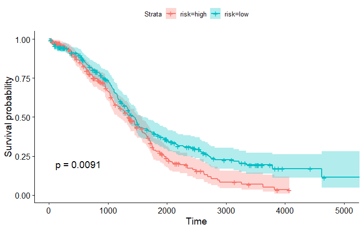
Section 4.2: Survival Analysis
Then, we perform survival analysis based on R package “survival” and “survminer”.
library(survival)
library(survminer)
library(tidyr)
library(gridExtra)

# import survival information
sur_info <- read.table(file = "Human__TCGA_OV__MS__Clinical__Clinical__01_28_2016__BI__Clinical__Firehose.tsi", header = TRUE, row.names = 1)
tmp_rowname <- rownames(sur_info)

data <- read.csv(file = "ov_ARIC.csv", header = TRUE, row.names = 1)

selected_celltype <- c("T.cells.CD8", "T.cells.gamma.delta",
                       "Macrophages.M1", "NK.cells.resting",
                       "NK.cells.activated")

data <- data[selected_celltype, ]
data <- colSums(x = data)
prop_median <- median(data)

high_risk <- names(data)[which(data <= prop_median)]
low_risk <- names(data)[which(data > prop_median)]

label <- rep(x = "tumor", times = ncol(sur_info))
names(label) <- colnames(sur_info)
idx_high <- which(names(label) %in% high_risk)
label[idx_high] <- "high"
idx_low <- which(names(label) %in% low_risk)
label[idx_low] <- "low"

sur_info <- rbind(sur_info, label)
rownames(sur_info) <- c(tmp_rowname, "risk")

sur_info <- as.data.frame(t(sur_info[, which(colnames(sur_info) %in% names(data))]))

sur_info <- drop_na(data = sur_info, c("overall_survival", "status"))
sur_info <- transform(sur_info, overall_survival = as.numeric(overall_survival))
sur_info <- transform(sur_info, status = as.numeric(status))

fit <- survfit(Surv(overall_survival, status) ~ risk, data=sur_info)
ggsurvplot(fit, pval = TRUE, conf.int = TRUE)

res_cox <- coxph(Surv(overall_survival, status) ~ risk, data=sur_info)

summary(res_cox)$conf.int
Then, we can get the survival curve and hazard ratio like below.
        exp(coef) exp(-coef) lower .95 upper .95
risklow 0.7424766   1.346844  0.593249 0.9292413
Section 5: Computational Efficiency Comparison
Computational efficiency is largely influenced by the number of markers. Therefore, we compared the computation time with both different methods and different marker numbers.
We generated in silico mixed gene expression data with different marker numbers (100, 500, 1000, 2000, 5000, 7000 and 10000). In order to get a reliable result, we generated 10 datasets and each dataset had 50 samples for each situation with different marker numbers. We compared the mean computation time for 50 samples and summarized the results in the foloowing table.
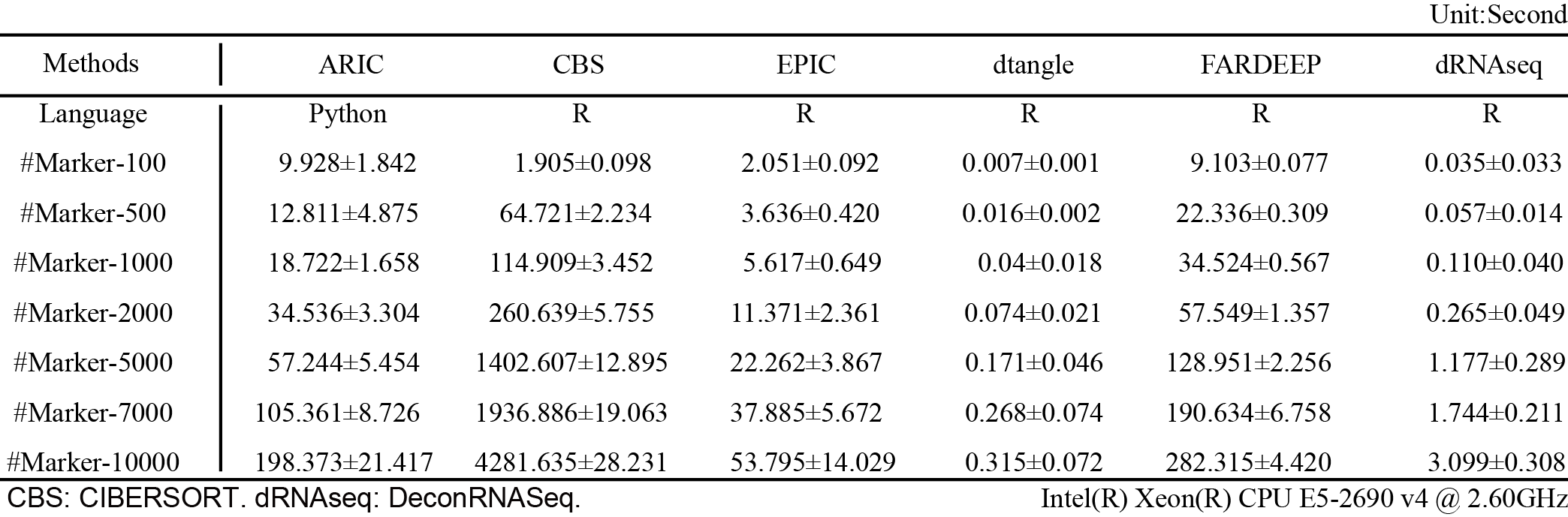
ARIC needs to compute component-wise condition number after removing each collinearity marker. Therefore, the computational time will be longer than matrix operation-based methods like dtangle and deconRNAseq. The computational efficiencies of ARIC, EPIC and FARDEEP are at the same level. In addition, computational time of CIBERSORT growth drastically with the increase of marker number. Thus, we strongly recommended filtering low quality markers before deconvolution.
Citation
Zhang, Wei, Hanwen Xu, Rong Qiao, Bixi Zhong, Xianglin Zhang, Jin Gu, Xuegong Zhang, Lei Wei, and Xiaowo Wang. “ARIC: accurate and robust inference of cell type proportions from bulk gene expression or DNA methylation data.” Briefings in Bioinformatics 23, no. 1 (2022): bbab362.